- Use similarity (0.7, 1) to form clusters
2. cut all clusters that have more than 20 features
3. use merged result on only articles with word count > 80
The original result is :0.7783
2. cut all clusters that have more than 20 features
3. use merged result on only articles with word count > 80
The original result is :0.7783
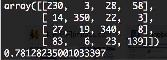
Confusion Matrix for original NB:
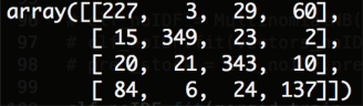
for NB with similarity in (0.8, 1)

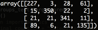
for NB with similarity in (0.7, 1)
Added stemmer: Feature size from 26879 to 25054, accuracy from
0.77848 to 0.77830
–with original Naive Bayes
Final: positiveCount: 582 zeroCount: 23395 oneCount: 13912 negativeCount: 17036552 l
max: 1.0
min: -0.303092024177
Non-stemmed: (0.9, 1)->160 (0.8, 0.9)->1570 (0.7, 0.8)8660 (0.6, 0.7)55896
Stemmed: (0.9, 1)->132 (0.8, 0.9)->1032 (0.7, 0.8)5040 (0.6, 0.7)41750
Non-stemmed: —>F1:0.77848
Clusters-in-(0.9-1): Num of clusters: 27, num of features: 77 —>F1: 0.7806
Clusters-in-(0.8-0.9): Num of clusters: 524, num of features: 1211 —>F1: 0.7754
Clusters-in-(0.7-0.8): Num of clusters: 1844, num of features: 5216 —>F1: 0.7771
Clusters-in-(0.6-0.7): Num of clusters: 1587, num of features: 10224 —>F1: 0.7525
Stemmed: —> F1: 0.77830
Clusters-in-(0.9-1): Num of clusters: 17, num of features: 54 —> F1: 0.77748
Clusters-in-(0.8-1): Num of clusters: 316, num of features: 746 —>F1: 0.778366
Clusters-in-(0.7-1): Num of clusters: 1122, num of features: 2982 —>F1: 0.77680
Clusters-in-(0.6-1): Num of clusters: 1444, num of features: 7659 —>F1: 0.75831
Word2Vec distance isn’t semantic distance
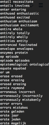
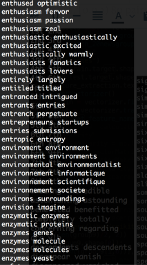
The Word2Vec metric tends to place two words close to each other if they occur in similar contexts— that is, w and w’ are close to each other if the words that tend to show up near w also tend to show up near w’ (This is probably an oversimplification, but see this paper of Levy and Goldberg for a more precise formulation.) If two words are very close to synonymous, you’d expect them to show up in similar contexts, and indeed synonymous words tend to be close:
>>> model.similarity(‘tremendous’,’enormous’)
0.74432902555062841
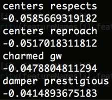
The notion of similarity used here is just cosine distance (which is to say, dot product of vectors.) It’s positive when the words are close to each other, negative when the words are far. For two completely random words, the similarity is pretty close to 0.
On the other hand:
>>> model.similarity(‘tremendous’,’negligible’)
0.37869063705009987
Tremendous and negligible are very far apart semantically; but both words are likely to occur in contexts where we’re talking about size, and using long, Latinate words. ‘Negligible’ is actually one of the 500 words closest to ’tremendous’ in the whole 3m-word database.
Original F1-score: 0.7785
use only >0.9 similarities,merged 77 features into 27 cluster-features, total from 26879 to 26829, F1-score: 0.7806
use only [0.8,0.9) similarities, merged 1211 features into 524 cluster-features, total from 26879 to 26192, F1-score: 0.7754
use only [0.7,0.8) similarities, merged 5216 features into 1844 cluster-features, total from 26879 to 23507, F1-score: 0.7771
use only[0.6,0.7) similarities, merged 10224 features into 1587 cluster-features, total from 26879 to 18242, F1-score: 0.7525
use >=0.7 similarities, merged features from 26879 to 23081, F1-score: 0.7754
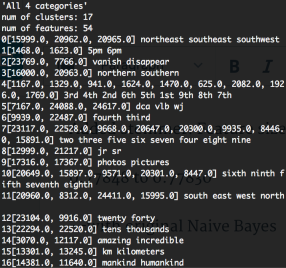
Investigation on 0.9 similarities group
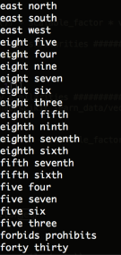
0 revenue revenues
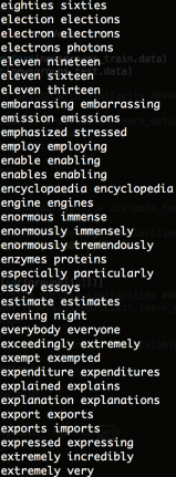
1 astounding astonishing
2 eighth seventh ninth sixth fifth
3 north west east south
4 concerning regarding
5 kilometers km kms
6 benefitted benefited
7 5pm 6pm
8 6th 8th 4th 7th 9th 5th 3rd 2nd 1st
9 southern northern
10 forty thirty twenty
11 wj vlb dca
12 descendents descendants
13 fourth third
14 jr sr
15 photos pictures
16 hundreds thousands tens
17 four seven five six three eight nine two
18 totally completely
19 predominantly predominately
20 incredible amazing
21 humankind mankind
22 disappeared vanished
23 forbids prohibits
24 northeast southeast southwest
25 disappear vanish
26 horrible terrible
By removing 9,17,and 20, we get the original 0.7785
Topic: Use Word2Vec to select feature
add up all features that have high similarity (>0.9)
 But, similar features are intertwined
–> Use graph search to identify all connected components:
–> add up weight for each group and become new features
Incorporate Word2Vec Similarity into Vectors
Issue
Analysis on Similarity Matrix:
38% Positive; 54% Zero; 8% Negative
Max: 2057.21140249
Min: 0.0
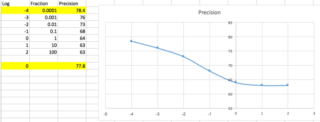
Use scale factor to tune the vectors:
vector = W +scale_factor * Wsimilarity
Result
categories: [‘alt.atheism’, ‘talk.religion.misc’, ‘comp.graphics’, ‘sci.space’]
training set: (2034,), testing set: (1353,)
Customized:
Count: 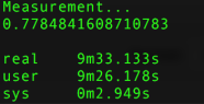
TF-IDF: 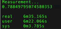
Original:
count: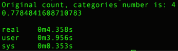
TF-IDF: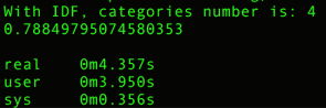
Build MNB using 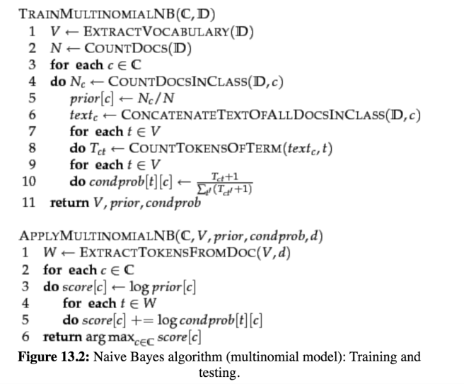
A working example is shown below:
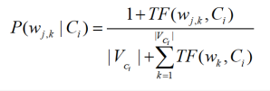
To eliminate zeros, we use add-one or Laplace smoothing, which simply adds one to each count (cf. Section 11.3.2 ):
where ![]() is the number of terms in the vocabulary. Add-one smoothing can be interpreted as a uniform prior (each term occurs once for each class) that is then updated as evidence from the training data comes in. Note that this is a prior probability for the occurrence of a term as opposed to the prior probability of a class which we estimate in Equation 116 on the document level.
is the number of terms in the vocabulary. Add-one smoothing can be interpreted as a uniform prior (each term occurs once for each class) that is then updated as evidence from the training data comes in. Note that this is a prior probability for the occurrence of a term as opposed to the prior probability of a class which we estimate in Equation 116 on the document level.
We have now introduced all the elements we need for training and applying an NB classifier. The complete algorithm is described in Figure 13.2 .
| docID | words in document | in |
|||
| training set | 1 | Chinese Beijing Chinese | yes | ||
| 2 | Chinese Chinese Shanghai | yes | |||
| 3 | Chinese Macao | yes | |||
| 4 | Tokyo Japan Chinese | no | |||
| test set | 5 | Chinese Chinese Chinese Tokyo Japan | ? |
Worked example. For the example in Table 13.1 , the multinomial parameters we need to classify the test document are the priors ![]() and
and ![]() and the following conditional probabilities:
and the following conditional probabilities:

The denominators are ![]() and
and ![]() because the lengths of
because the lengths of ![]() and
and ![]() are 8 and 3, respectively, and because the constant
are 8 and 3, respectively, and because the constant ![]() in Equation 119 is 6 as the vocabulary consists of six terms.
in Equation 119 is 6 as the vocabulary consists of six terms.
We then get:

Thus, the classifier assigns the test document to ![]() = China. The reason for this classification decision is that the three occurrences of the positive indicator Chinese in
= China. The reason for this classification decision is that the three occurrences of the positive indicator Chinese in ![]() outweigh the occurrences of the two negative indicators Japan and Tokyo. End worked example.
outweigh the occurrences of the two negative indicators Japan and Tokyo. End worked example.
DataSet
1. Text categorization Benchmark
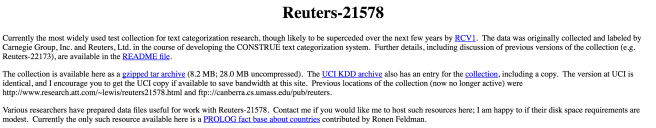
1. Reuters-21578 –> 21,578 docs, 135 different topics
http://www.daviddlewis.com/resources/testcollections/reuters21578/
2. 20 Newsgroups –>20,000 docs, 20 different topics
http://qwone.com/~jason/20Newsgroups/

2. Practical text categorization
Literature
Proposed Project Name
Categorize Text with Naive Bayes and word2vec word embedding
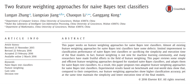
Literature Review
DataSet
yelp review –> based on review to predict business category
pros: easy to get dataset;
cons: the business category seems to be obvious
Twitter thread –> based on thread content to predict the category
pros: makes more sense of category prediction
cons: hard to get labeled dataset;
Implementation Plan
